Student name: Zhiqiang Sun
Student pace: self paced
Business understanding
The skin cancer dataset contains many medical images that show various kinds of skin cancer. In this project, we will analyze and visualize the relationship between cancer and age and the location of the body. Furthermore, we will use machine learning to train a model that can distinguish the cancer type by given images.
Dataset
The whole dataset were download from kaggle (https://www.kaggle.com/code/rakshitacharya/skin-cancer-data/data). The folder contains several csv files and two images folder. All the name of images were named with image id which can be found in the metadata excel file. There are several other hinist csv file which include the pixels information of corresponding images in different resolusion. In this project, we will focus on the information from the metadata. Also, when we creat the model, we will use the original images for higher resolusion, thus we will dismiss all the hmnist data this time.
The data has seven different classes of skin cancer which are listed below :
- Melanocytic nevi
- Melanoma
- Benign keratosis-like lesions
- Basal cell carcinoma
- Actinic keratoses
- Vascular lesions
- Dermatofibroma
In this project, I will try to train a model of 7 different skin cancer classes using Convolution Neural Network with Keras TensorFlow and then use it to predict the types of skin cancer with random images. Here is the plan of the project step by step:
- Import all the necessary libraries for this project
- Make a dictionary of images and labels
- Reading and processing the metadata
- Process data cleaning
- Exploring the data analysis
- Train Test Split based on the data frame
- Creat and transfer the images to the corresponding folders
- Do image augmentation and generate extra images to the imbalanced skin types
- Do data generator for training, validation, and test folders
- Build the CNN model
- Fitting the model
- Model Evaluation
- Visualize some random images with prediction
1. Import all the necessary libraries for this project
# import the necessary libraries for this project
import pandas as pd
import matplotlib.pyplot as plt
import numpy as np
import os, shutil
from glob import glob
from sklearn.model_selection import train_test_split
from keras.preprocessing.image import ImageDataGenerator
from tensorflow.keras.applications import VGG19, inception_resnet_v2, xception
from tensorflow.keras import layers
from tensorflow.keras.layers import Dropout
from tensorflow.keras import models
from tensorflow.keras import optimizers
import matplotlib.pyplot as plt
from sklearn.metrics import classification_report,confusion_matrix
import seaborn as sns

# import the libraries for dash plot
from jupyter_dash import JupyterDash
import dash
from dash import dcc
from dash import html
import pandas as pd
import plotly.express as px
from dash.dependencies import Input, Output
app = JupyterDash(__name__)
server = app.server
2. Make a dictionary of images and labels
In this steps, I make the path for all the images and a dictionary for all types of skin cancers with full names.
path_dict = {os.path.splitext(os.path.basename(x))[0] :x for  x in glob(os.path.join('*', '*.jpg'))}
lesion_type_dict = {
    'nv': 'Melanocytic nevi',
    'mel': 'Melanoma',
    'bkl': 'Benign keratosis-like lesions ',
    'bcc': 'Basal cell carcinoma',
    'akiec': 'Actinic keratoses',
    'vasc': 'Vascular lesions',
    'df': 'Dermatofibroma'
}
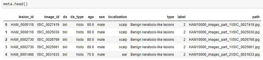
3. Reading and processing the metadata
In this step, we have read the csv which had the information for all the patients and images. Afterthat, we made three more columns including the cancer type in full name, the label in skin cancers in digital and the path of image_id in the folder.
# read the metadata
meta = pd.read_csv('HAM10000_metadata.csv')

# generate new columns of type, lebel and path
meta['type'] = meta['dx'].map(lesion_type_dict.get)
meta['label'] = pd.Categorical(meta['type']).codes
meta['path'] = meta['image_id'].map(path_dict.get)
meta.head()
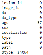
4. Process data cleaning
In this part, we check the missing values for each column and fill them.
meta.isna().sum()
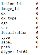
# fill the missing age with their mean.
meta['age'].fillna((meta['age'].mean()), inplace=True)
meta.isna().sum()
5. Exploring the data analysis
In this part, we briefly explored different features of the dataset, their distributions and counts.
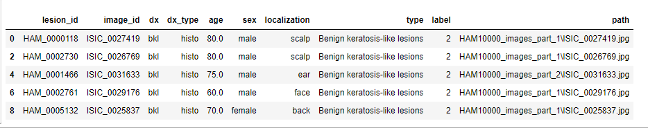
As there is some duplecate lesion_id which belong to same patient, all the features except the image_id for them are same with each other. Thus, we first find and remove the duplex.
# compare the unique values for lesion id and image id.
meta.lesion_id.nunique(), meta.image_id.nunique()
(7470, 10015)
# drop the duplication based on the lesion_id.
meta_patient = meta.drop_duplicates(subset=['lesion_id'])

meta_patient.head()
# plot distribution of features 'dx', 'dx_type',  'sex', 'localization'.
feat = ['dx', 'dx_type',  'sex', 'localization']
plt.subplots(figsize=(11, 8))
for i, fea in enumerate(feat):
    length = len(feat)
    plt.subplot(2, 2, i+1)
    meta_patient[fea].value_counts().plot.bar(fontsize = 10)
    plt.ylabel('counts', fontsize = 15)
    plt.xticks()
    plt.title(fea, fontsize = 15)
    plt.tight_layout()
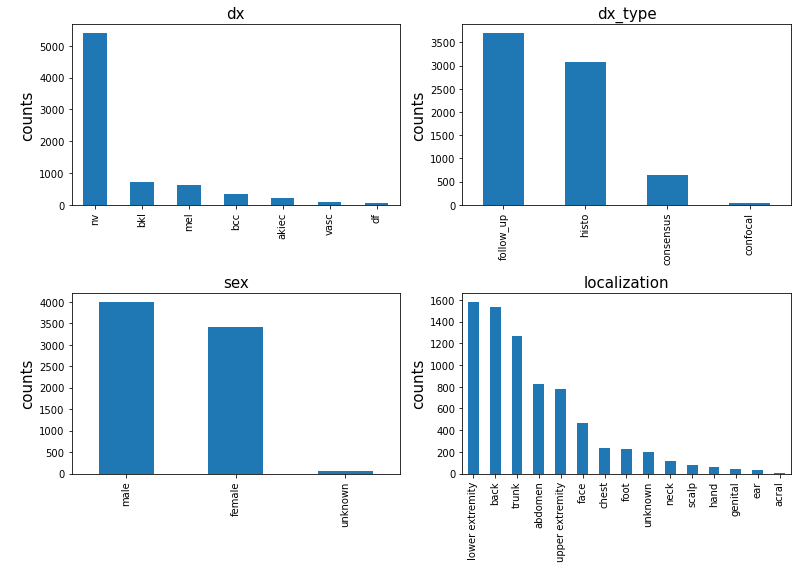
We checked the distribution of columns ‘dx’, ‘dx_type’, ‘sex’, ‘localization’ for different patients. The graphs show that:
- In dx features, the ‘nv’: ‘Melanocytic nevi’ case take more than 70% of the total cases. The number suggests that this dataset is an unbalanced dataset.
- In dx_type features, the histogram suggests most of the cancer were confirmed in Follow-up and histo Histopathologic diagnoses.
- The sex feature shows that the amount of male who had skin cancer is slight larger than female but still similar to each other.
- The localization analysis shows that lower extremity, back ,trunk abdomen and upper extremity are heavily compromised regions of skin cancer
# Creat dashboard to visualize the distribution of age for different types of skin cancer

app.layout = html.Div(children=[
    html.H1(children='Distribution of Age', style={'text-align': 'center'}),


    html.Div([
        html.Label(['Choose a graph:'],style={'font-weight': 'bold'}),
        dcc.Dropdown(
            id='dropdown',
            options=[
                {'label': 'all types', 'value': 'all'},
                {'label': 'nv', 'value': 'nv'},
                {'label': 'bkl', 'value': 'bkl'},
                {'label': 'mel', 'value': 'mel'},
                {'label': 'bcc', 'value': 'bcc'},
                {'label': 'akiec', 'value': 'akiec'},
                {'label': 'vasc', 'value': 'vasc'},
                {'label': 'df', 'value': 'df'}
                    ],
            value='all types',
            style={"width": "60%"}),

    html.Div(dcc.Graph(id='graph')),
        ]),

])

@app.callback(
    Output('graph', 'figure'),
    [Input(component_id='dropdown', component_property='value')]
)
def select_graph(value):
    if value == 'all':
        fig = px.histogram(None , x= meta_patient['age'], nbins=20, labels={'x':value, 'y':'count'})

        return fig
    else:
        fig = px.histogram(None , x= meta_patient[meta_patient['dx'] == value]['age'],
                           nbins=20,  labels={'x':value, 'y':'count'})

        return fig

if __name__ == '__main__':
    app.run_server(mode = 'inline')

In general, most cancers happen between 35 to 70. Age 45 is a high peak for patients to get a skin cancer. Some types of skin cancer (vasc, nv) happen to those below 20, and others occur most after 30.
6. Train Test Split based on the data frame
We split the dataset to training (70%), validation (10%) and testing (20%) by train_test_split.
df = meta.drop(columns='label')
target = meta['label']
X_train_a, X_test, y_train_a, y_test = train_test_split(df, target, test_size=0.2, random_state=123)
X_train, X_val, y_train, y_val = train_test_split(X_train_a, y_train_a, test_size=0.1, random_state=12)
X_train.shape, X_val.shape, X_test.shape
((7210, 9), (802, 9), (2003, 9))
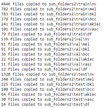
**7. Creat and transfer the images to the corresponding folders **
We created the subfolders containing the train, Val, and test folder. In addition, we created a folder for all types of skin cancers in each of the folders. Finally, We transferred the images to the corresponding folder based on the data frame and the path in each image ID.
# copy the images to correct folder according to the image_id in dataframe

new_dir = 'sub_folders2'
os.makedirs(new_dir)  # creat the subfolders
TVT = ['train', 'val', 'test']
lesion = lesion_type_dict.keys()
for first in TVT:
    temp_dir = os.path.join(new_dir, first)
    os.mkdir(temp_dir) # creat the train, val and test folders

    for sec in lesion:
        sec_dir = os.path.join(temp_dir, sec)
        os.mkdir(sec_dir) # creat the subfolders of all tpyes of cancers

        if first == 'train':
            source_df = X_train[X_train['dx'] == sec] # find the source of train dataset
        if first == 'val':
            source_df = X_val[X_val['dx'] == sec] # find the source of validation dataset
        elif first == 'test':
            source_df = X_test[X_test['dx'] == sec] # find the source of test dataset


        for source in source_df.path: # find the images to transfer
            shutil.copy(source, sec_dir)
        print("{} files copied to {}".format(len(source_df.path), sec_dir))
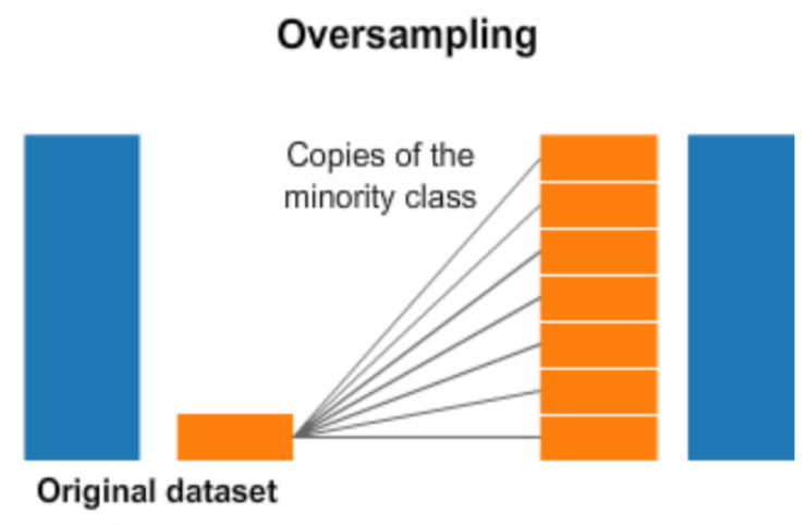
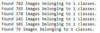
8. Do image augmentation and generate extra images to the imbalanced skin types
The amounts of files in each training folder type tell us the images of nv are much higher than others. The imbalance of the training dataset might cause a high bias in model fitting. Thus we will generate some more images for other kinds of cancers. Here we use image augmentation to oversample the samples in all classes except nv. Here is a simple chart about the oversampling.
# We only need to fill more images to all class except nv
class_list = ['mel','bkl','bcc','akiec','vasc','df']

for cat in class_list:
    # creat temp folder for augmentaion
    temp_dir = 'temp'
    os.mkdir(temp_dir)
    img_dir = os.path.join(temp_dir, cat)
    os.mkdir(img_dir)

    # copy the original images to temperate folder
    img_list = os.listdir('sub_folders2/train/'+cat)

    for image in img_list:
        source = os.path.join('sub_folders2/train/'+cat, image)
        dest = os.path.join(temp_dir)
        shutil.copy(source,img_dir)

    path = temp_dir
    save_path = 'sub_folders2/train/'+cat
    # set the parameters of image augmentation
    data_datagen = ImageDataGenerator(rescale=1./255,
                                       rotation_range=180, # randomly rotate images in the range (degrees, 0 to 180)
                                       width_shift_range=0.2, # randomly shift images horizontally (fraction of total width)
                                       height_shift_range=0.2, # randomly shift images vertically (fraction of total height)
                                       shear_range=0.2,# Randomly shear image
                                       zoom_range=0.2, # Randomly zoom image
                                       horizontal_flip=True, # randomly flip images
                                       vertical_flip=True,# randomly flip images
                                       fill_mode='nearest')


    batch_size = 50

    temp_generator = data_datagen.flow_from_directory(path,
                                                      save_to_dir = save_path,
                                                      save_format = 'jpg',
                                                      target_size = (224, 224),
                                                      batch_size=batch_size
                                                        )
    # Generate the temp images and add them to the training folders

    num_needed = 5000
    num_cur =  len(os.listdir(img_dir))
    num_batches = int(np.ceil((num_needed - num_cur)/batch_size))

    for i in range (0, num_batches):
        imgs, label = next(temp_generator)
    # delete the temp folders after each transfer
    shutil.rmtree(temp_dir)
# check the files in each of the folders after image augmentation
class_list = ['nv', 'mel','bkl','bcc','akiec','vasc','df']

for cat in class_list:
    print(len(os.listdir('sub_folders/train/'+cat)))
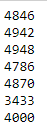
The numers of files in each folders are in same levels.
9. Do data generator for training, validation, and test folders
new_dir = 'sub_folders2/'
train_dir = '{}train'.format(new_dir)
validation_dir = '{}val/'.format(new_dir)
test_dir = '{}test/'.format(new_dir)

batch_size = 50
image_size = 224

data_datagen = ImageDataGenerator(rescale=1./255,
                                   rotation_range=180 ,# randomly rotate images in the range (degrees, 0 to 40)
                                   width_shift_range=0.2,# randomly shift images horizontally (fraction of total width)
                                   height_shift_range=0.2,# randomly shift images vertically (fraction of total height)
                                   shear_range=0.2,
                                   zoom_range=0.2, # Randomly zoom image
                                   horizontal_flip=True, # randomly flip images
                                   vertical_flip=True, # randomly flip images
                                   fill_mode='nearest')


train_generator = ImageDataGenerator(rescale=1./255).flow_from_directory(train_dir,
                                                    target_size=(image_size, image_size),
                                                    batch_size= batch_size,
                                                    class_mode='categorical')


val_generator = ImageDataGenerator(rescale=1./255).flow_from_directory(validation_dir,
                                                target_size=(image_size, image_size),
                                                batch_size=batch_size,
                                                class_mode='categorical')

test_generator = ImageDataGenerator(rescale=1./255).flow_from_directory(test_dir,
                                                target_size=(image_size, image_size),
                                                batch_size=1,
                                                class_mode='categorical',
                                                shuffle=False)
Found 31825 images belonging to 7 classes.
Found 802 images belonging to 7 classes.
Found 2003 images belonging to 7 classes.
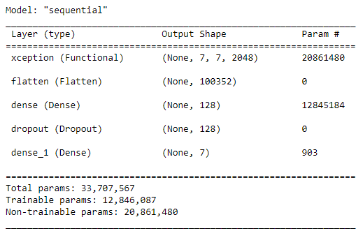
** 10. Build the CNN model**
WE build a CNN model base on the pretrained model ‘xception’.
cnn_base_xception = xception.Xception(weights='imagenet',
                 include_top=False,
                 input_shape=(224, 224, 3))

# Define Model Architecture
model = models.Sequential()
model.add(cnn_base_xception)
model.add(layers.Flatten())

model.add(layers.Dense(128, activation='relu'))
model.add(Dropout(0.2))  # dropout 25% of the nodes to prevent overfitting
model.add(layers.Dense(7, activation='softmax'))

cnn_base_xception.trainable = False

model.summary()
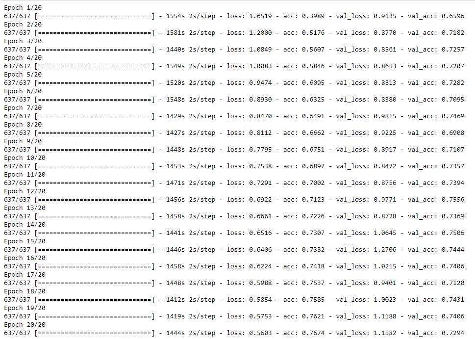
11. Fitting the model
We fit the training data to the model we created earlier
# find out the numbers of trainning and validation
num_train = len(train_generator.labels)
num_val = len(val_generator.labels)
train_steps = np.ceil(num_train/batch_size)
val_steps = np.ceil(num_val/batch_size)
# compile and fit the model with training dataset
model.compile(loss='categorical_crossentropy',
               # set the optimizer
              optimizer=optimizers.Adam(learning_rate=0.001, beta_1=0.9, beta_2=0.999, epsilon=None, decay=0.0, amsgrad=False),
              metrics=['acc'])

history = model.fit(train_generator,
                              steps_per_epoch=train_steps,
                              epochs=20,
                              validation_data=val_generator,
                              validation_steps=val_steps)
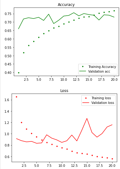
# Plot the accuracy and loss for train and validation.
def plot_acc(history):
    train_acc = history.history['acc']
    val_acc = history.history['val_acc']
    train_loss = history.history['loss']
    val_loss = history.history['val_loss']
    epch = range(1, len(train_acc) + 1)
    plt.plot(epch, train_acc, 'g.', label='Training Accuracy')
    plt.plot(epch, val_acc, 'g', label='Validation acc')
    plt.title('Accuracy')
    plt.legend()
    plt.figure()
    plt.plot(epch, train_loss, 'r.', label='Training loss')
    plt.plot(epch, val_loss, 'r', label='Validation loss')
    plt.title('Loss')
    plt.legend()
    plt.show()
plot_acc(history)
#save the model
model.save('results_on_xception_final_2.h5')
12. Model Evaluation
In this step we will check the testing accuracy and validation accuracy of our model,plot confusion matrix and also check the missclassified images count of each type.
# evaluate the model with test dataset.
test_loss, test_acc = model.evaluate(test_generator, steps=2003)

The accuracy of the model is 74.84% which is not bad at all.
# generate the prediction and true value of y
Y_pred = model.predict(test_generator)
Y_pred_classes = np.argmax(Y_pred,axis = 1)
Y_true = test_generator.labels
# make teh confusion matrix
confusion_mtx = confusion_matrix(Y_true, Y_pred_classes)
confusion_mtx
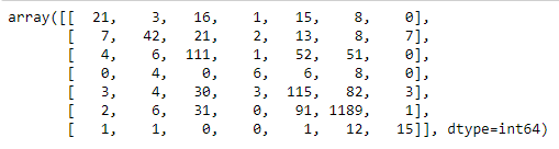
indices = test_generator.class_indices
# plot the confusion matrix
plt.figure(figsize=(15,8))
def plot_confusion_matrix(mtx, indices, normalize = False, title = 'confusion matrix', cmap = plt.cm.Reds):
    plt.imshow(mtx, interpolation='nearest', cmap = cmap)
    plt.title = title
    plt.colorbar()
    tick_mark = np.arange(len(indices))
    plt.xticks (tick_mark, indices.keys(),  fontsize = 13)
    plt.yticks (tick_mark, indices.keys(), fontsize = 13)

    if normalize:
        mtx = mtx/mtx.sum(axis = 1)[:,np.newaxis]


    for i in range(mtx.shape[0]):
        for j in range(mtx.shape[1]):
            plt.text(j,i,mtx[i][j], horizontalalignment = 'center', fontsize = 15)
    plt.tight_layout()
    plt.ylabel('True label', fontsize = 15)
    plt.xlabel('Predicted label', fontsize = 15)

plot_confusion_matrix(confusion_mtx, indices = indices)

print(classification_report(Y_true,Y_pred_classes,target_names =['akiec', 'bcc', 'bkl','df', 'mel', 'nv','vasc' ]))
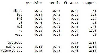
The f1 score for nv class is highest and over 0.88. The f1-score on df, akiec and mel are less than 0.5 which sugessted that the prediction on these three type are less accurate.
# plot the mistypes of prediction for every class
label_frac_error = 1 - np.diag(confusion_mtx) / np.sum(confusion_mtx, axis=1)
plt.bar(np.arange(7),label_frac_error)
plt.xlabel('True Label')
tick_mark = np.arange(len(indices))
plt.xticks (tick_mark, indices.keys(),  fontsize = 13)
plt.ylabel('Fraction classified incorrectly')
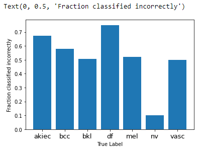
It seems that the maximum number of incorrect predicitons are features mel and then df and akiec. The nv has least misclassified type.
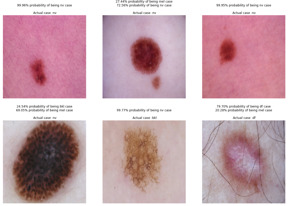
# ramdomly plot images in testing folder with the predicted and true case.
test_generator.reset()
x=np.concatenate([test_generator.next()[0] for i in range(test_generator.__len__())])
y=np.concatenate([test_generator.next()[1] for i in range(test_generator.__len__())])
#print(x.shape)
#print(y.shape)
dic = { 0 : 'akiec', 1: 'bcc', 2: 'bkl',3: 'df', 4: 'mel',5: 'nv',6: 'vasc'}
plt.figure(figsize=(20,14))

#for i in range(0+200, 9+200):
for idx, i in enumerate(np.random.randint(1, 2003, 6)):
    plt.subplot(2, 3, idx+1)
    out = str()
    for j in range(0,6):
        if Y_pred[i][j] > 0.1:
            out += '{:.2%} probability of being {} case'.format(Y_pred[i][j], dic[j]) + '\n'
        #else: out = 'None'


    plt.title(out +"\n Actual case :" + dic[Y_true[i]])
    plt.imshow(np.squeeze(x[i]))
    plt.axis('off')
plt.show()
Conclusion
We can extract the information about skin cancer from the metadata and explore the distribution of various features. For example, the most often age of skin cancer occur is around 45. We make one CNN model which can fit and predict the type of skin cancer well based on the images. The accuracy is 74.9% which is more efficient than detection with human eyes.