Overview
For this project, we trained a pretrained cnn model to predict the Classification of the x-ray images.
Business understanding
The medical dataset comes from Kermany et al. contains a set of x-ray images of pediatric patients. The images will show whether the patients have pneumonia or not. Our task is to build a model that can classify whether a given patient has pneumonia given a chest x-ray image. Since this is an Image Classification problem, we will solve it with Deep Learning.
The Dataset
The dataset that we will use for image classification is the chese_xray which contains two categories: Pneumonia and Normal. The data was downloaded from https://data.mendeley.com/datasets/rscbjbr9sj/3 to the local drive and unzipped. The data set is assigned into two folders (train and test) and contains a subfolder for each Pneumonia and Normal category. In each of the folders, there are a lot of x-ray images. To check how many samples were in each category, we used the OS.listdir methods.
# load all the necessary libraries
import numpy as np
import os, shutil
import pandas as pd
from keras.preprocessing.image import ImageDataGenerator
from tensorflow.keras.applications import VGG19
from tensorflow.keras import layers
from tensorflow.keras import models
from tensorflow.keras import optimizers
import matplotlib.pyplot as plt
from sklearn.metrics import classification_report,confusion_matrix
import seaborn as sns
list_train_normal = os.listdir('chest_xray/train/normal')
list_train_PNEUMONIA = os.listdir('chest_xray/train/PNEUMONIA')
list_test_normal = os.listdir('chest_xray/test/normal')
list_test_PNEUMONIA = os.listdir('chest_xray/test/PNEUMONIA')


len(list_train_normal), len(list_train_PNEUMONIA), len(list_test_normal), len(list_test_PNEUMONIA)
(1349, 3884, 235, 390)
IIn the train folder, there is a regular folder that contains 1349 images and the PNEUMONIA folder, which includes 3884 images. The NORMAL folder in the test folder contains 235 pictures, and the PNEUMONIA folder contains 390 images. The images in each folder are too large for the modeling since our local computer is not very powerful for multiple testing. Therefore, we need to downsample the dataset to find the optimal model and parameter first. We are then using the entire dataset to train and test our model. Based on our earlier experience, we will use 20% of the total dataset to model our model. We also need to make 10% of the training data to the validation dataset.
Plan
- Downsampleing the data set by randomly choosing 20% of the initial training and testing images to the new data_org_subset folder. Make a new validation folder and randomly select 5% of the pictures from the training folder.
- Define the trained generator, validation generator, and test generator.
- Build a baseline model.
- Build the deep learning model base on the Pretrained CNN (VGG19) by adding a few fully connected layers. Then, train the model with selected images.
- Retrain the model with complete training data.
- Evaluate the model with the test images.
1. Rebuild the data subset folder with 20% of the original images
# define the old and new direction of dataset

# define a new method to transfer the images between two folder
def transfer(no_of_files, source, dest):
    for i in range(no_of_files):
        #Variable random_file stores the name of the random file chosen
        random_file=np.random.choice(os.listdir(source))
        # print("%d} %s"%(i+1,random_file))
        source_file="%s/%s"%(source,random_file)
        dest_file=dest
        #"shutil.move" function moves file from one directory to another
        shutil.copy(source_file,dest_file)


# set the  propotion of images transfered to the new folders p_val, p_train, p_test and
# define a new method to creat and transfer images
def make_subset (old_dir, new_root_dir, p_val, p_train, p_test) :

    # make the root dir folder
    os.mkdir(new_root_dir)

    # define the name of subset to save all the images in different categories
    dir_names = ['train', 'val', 'test']
    cat_names = ['normal', 'PNEUMONIA']
    for d in dir_names:

        new_dir = os.path.join(new_root_dir, d)
        os.mkdir(new_dir)

        # make the source dir to train and test folder, since we donot have validation in the original folder,
        # we make it to train folder
        if d == 'val':
            source_dir = os.path.join(old_dir, 'train')
        else:
            source_dir = os.path.join(old_dir, d)


        for cat in cat_names:
            new_cat = os.path.join(new_dir, cat)
            source = os.path.join(source_dir, cat )
            os.mkdir(new_cat)
            no_of_files = len(os.listdir(source))
            # set the nunmber of copy to 20% from source folder. For the validation folder, copy 5% of the images of source
            if d == 'val':
                no_of_copy = int(p_val * no_of_files)

            if d == 'train':
                no_of_copy = int(p_train * no_of_files)

            if d == 'test':
                no_of_copy = int(p_test * no_of_files )

            #print('d = ', d)
            print('copy {} of files in {} total files  from {} to {}'.format(no_of_copy,no_of_files, source, new_cat))
            transfer(no_of_copy, source, new_cat)

old_dir = 'chest_xray/'
new_root_dir = 'data_org_subset/'
make_subset(old_dir, new_root_dir, p_val = 0.05, p_train = 0.2, p_test = 0.2)
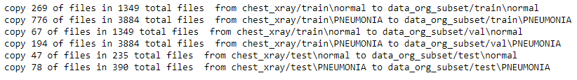
We copied 20% of the training and testing images from the original folder. We also made a new folder for validation and randomly selected 5% of the images from the training folder.
2. Define the train generator, validation generator and test generator.
# define the direction for train , vlalidation and test folder

train_dir = '{}train'.format(new_root_dir)
validation_dir = '{}val/'.format(new_root_dir)
test_dir = '{}test/'.format(new_root_dir)

train_datagen = ImageDataGenerator(rescale=1./255,
                                   rotation_range=40,
                                   width_shift_range=0.2,
                                   height_shift_range=0.2,
                                   shear_range=0.2,
                                   zoom_range=0.2,
                                   horizontal_flip=True,
                                   fill_mode='nearest')


train_generator = train_datagen.flow_from_directory(train_dir,
                                                    target_size=(300, 300),
                                                    batch_size= 20,
                                                    class_mode='categorical')

# Get all the data in the directory split/validation (200 images), and reshape them
val_generator = ImageDataGenerator(rescale=1./255).flow_from_directory(validation_dir,
                                                                       target_size=(300, 300),
                                                                       batch_size=20,
                                                                       class_mode='categorical')
Found 957 images belonging to 2 classes.
Found 255 images belonging to 2 classes.
# plotsome of the train set images we resampled in the train dataset
plt.figure(figsize=(12, 8))
for i in range(0, 8):
    plt.subplot(2, 4, i+1)
    for X_batch, Y_batch in train_generator:
        image = X_batch[0]
        dic = {0:'NORMAL', 1:'PNEUMONIA'}
        plt.title(dic[Y_batch[0][0]])
        plt.axis('off')
        plt.imshow(np.squeeze(image),cmap='gray',interpolation='nearest')
        break
plt.tight_layout()
plt.show()
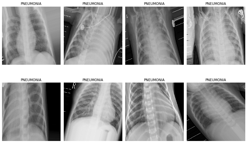
We plot some of the images in the training dataset. However, I can not tell which one is a case of pneumonia and which one is a normal case just by looking at the pictures. So now we will train the computer with a Pretrainned CNN model to predict whether the picture belongs to pneumonia or normal case.
3. Build a baseline model
model = models.Sequential()
model.add(layers.Conv2D(32, (3, 3), activation='relu',
input_shape=(300, 300, 3)))
model.add(layers.MaxPooling2D((2, 2)))
model.add(layers.Conv2D(64, (3, 3), activation='relu'))
model.add(layers.MaxPooling2D((2, 2)))
model.add(layers.Conv2D(128, (3, 3), activation='relu'))
model.add(layers.MaxPooling2D((2, 2)))
model.add(layers.Conv2D(128, (3, 3), activation='relu'))
model.add(layers.MaxPooling2D((2, 2)))
model.add(layers.Flatten())
model.add(layers.Dense(64, activation='relu'))
model.add(layers.Dense(128, activation='relu'))
model.add(layers.Dense(256, activation='relu'))
model.add(layers.Dense(512, activation='relu'))
model.add(layers.Dense(2, activation='softmax'))
model.compile(loss='categorical_crossentropy',
optimizer=optimizers.RMSprop(lr=1e-4),
metrics=['acc'])
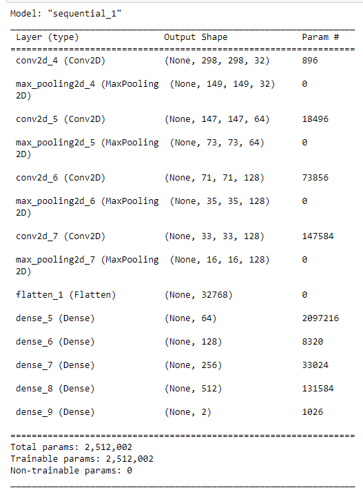
model.summary()
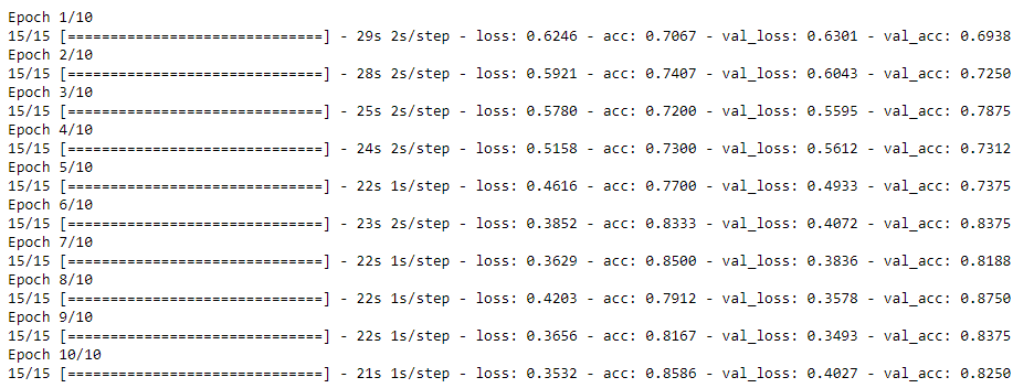
history = model.fit(train_generator,
                              steps_per_epoch=15,
                              epochs=10,
                              validation_data=val_generator,
                              validation_steps=8)
# Plot the accuracy and loss for train and validation.
def plot_acc(history):
    train_acc = history.history['acc']
    val_acc = history.history['val_acc']
    train_loss = history.history['loss']
    val_loss = history.history['val_loss']
    epch = range(1, len(train_acc) + 1)
    plt.plot(epch, train_acc, 'g.', label='Training Accuracy')
    plt.plot(epch, val_acc, 'g', label='Validation acc')
    plt.title('Accuracy')
    plt.legend()
    plt.figure()
    plt.plot(epch, train_loss, 'r.', label='Training loss')
    plt.plot(epch, val_loss, 'r', label='Validation loss')
    plt.title('Loss')
    plt.legend()
    plt.show()
plot_acc(history)

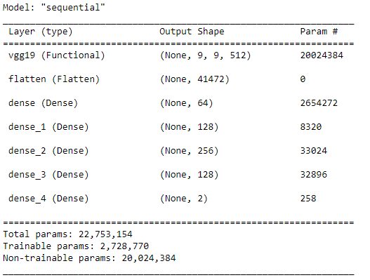
4. Build the model base on pretrain network VGG19.
# defined the pretrained model VGG19 and add more layer to the network.
cnn_base = VGG19(weights='imagenet',
                 include_top=False,
                 input_shape=(300, 300, 3))

# Define Model Architecture
model = models.Sequential()
model.add(cnn_base)
model.add(layers.Flatten())
model.add(layers.Dense(64, activation='relu'))
model.add(layers.Dense(128, activation='relu'))
model.add(layers.Dense(256, activation='relu'))
model.add(layers.Dense(128, activation='relu'))
model.add(layers.Dense(2, activation='softmax'))

cnn_base.trainable = False

model.summary()
# Compilation
model.compile(loss='categorical_crossentropy',
              optimizer=optimizers.RMSprop(learning_rate=2e-5),
              metrics=['acc'])

# Fitting the Model
history = model.fit(train_generator,
                              steps_per_epoch=15,
                              epochs=10,
                              validation_data=val_generator,
                              validation_steps=8)
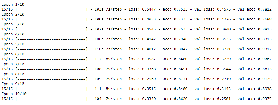
Now, we plot the accuracy and loss curve of the model to traning dataset.
#

train_acc = history.history['acc']
val_acc = history.history['val_acc']
train_loss = history.history['loss']
val_loss = history.history['val_loss']
epch = range(1, len(train_acc) + 1)
plt.plot(epch, train_acc, 'g.', label='Training Accuracy')
plt.plot(epch, val_acc, 'g', label='Validation acc')
plt.title('Accuracy')
plt.legend()
plt.figure()
plt.plot(epch, train_loss, 'r.', label='Training loss')
plt.plot(epch, val_loss, 'r', label='Validation loss')
plt.title('Loss')
plt.legend()
plt.show()
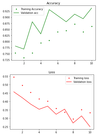
The acc and loss curve of training gave us a pretty good score, and the validation scores are going to a similar range in each step. Thus, we can use the same model for better training on the entire training dataset.
Save model
#
model.save('results_on_partial_dataset.h5')
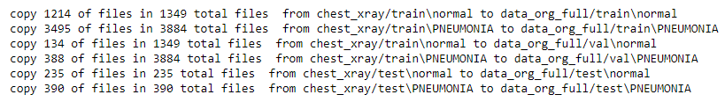
5. Retrain the model with full dataset.
Now is the time to use our model for the full dataset. We remade the folder of train, val, test folder for full dataset. Transfer 90% of train images to new train and 10% of train images to new validation folder. Transfer 100% of test to new test folder
old_dir = 'chest_xray/'
new_root_dir = 'data_org_full/'
make_subset(old_dir, new_root_dir, p_val = 0.1, p_train = 0.9, p_test = 1)
train_dir = '{}train'.format(new_root_dir)
validation_dir = '{}val/'.format(new_root_dir)
test_dir = '{}test/'.format(new_root_dir)

full_train_datagen = ImageDataGenerator(rescale=1./255,
                                   rotation_range=40,
                                   width_shift_range=0.2,
                                   height_shift_range=0.2,
                                   shear_range=0.2,
                                   zoom_range=0.2,
                                   horizontal_flip=True,
                                   fill_mode='nearest')


full_train_generator = full_train_datagen.flow_from_directory(train_dir,
                                                    target_size=(300, 300),
                                                    batch_size= 20,
                                                    class_mode='categorical')

# Get all the data in the directory split/validation (, and reshape them
full_val_generator = ImageDataGenerator(rescale=1./255).flow_from_directory(validation_dir,
                                                                       target_size=(300, 300),
                                                                       batch_size=20,
                                                                       class_mode='categorical')
Found 3132 images belonging to 2 classes.
Found 492 images belonging to 2 classes.
# recompile the model and fit to the full training dataset.
model.compile(loss='categorical_crossentropy',
optimizer=optimizers.RMSprop(learning_rate=2e-5),
metrics=['acc'])
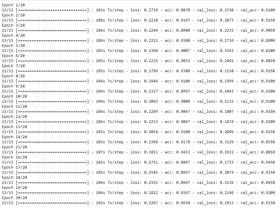
history = model.fit(full_train_generator,
steps_per_epoch=15,
epochs=20,
validation_data=full_val_generator,
validation_steps=10)
#save model
model.save('results_on_full_dataset.h5')
Plot the accuracy of the model again.
plot_acc(history)
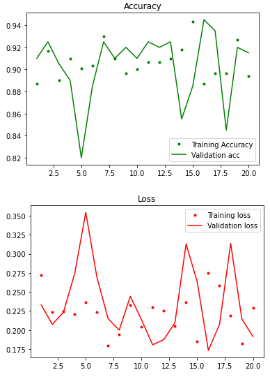
In this fitting, both training accuracy and validation accuracy are very high. Even though the fluctuation of validation accuracy is bigger than training accuracy, both accuracies generally had the same trend.
6. Evaluate the model with the test images.
We first generate the test labels as the real class of the images.
# Get all the data in the directory split/test (180 images), and reshape them


test_generator = ImageDataGenerator(rescale=1./255).flow_from_directory(test_dir,
                                                                        target_size=(300, 300),
                                                                        batch_size=399,
                                                                        class_mode='categorical',
                                                                        shuffle=False)


# generate the test_labels which is the y_true data
test_images, test_labels = next(test_generator)
We then calculated the accuracy of the model on the testing images.
test_datagen = ImageDataGenerator(rescale=1./255,
                                   rotation_range=40,
                                   width_shift_range=0.2,
                                   height_shift_range=0.2,
                                   shear_range=0.2,
                                   zoom_range=0.2,
                                   horizontal_flip=True,
                                   fill_mode='nearest')
test_generator2 = test_datagen.flow_from_directory(test_dir,
                                                  target_size=(300, 300),
                                                  batch_size=20,
                                                  class_mode='categorical',
                                                  shuffle=False)

test_loss, test_acc = model.evaluate(test_generator2, steps=10)
Found 399 images belonging to 2 classes.
10/10 [=====] - 42s 4s/step - loss: 0.0685 - acc: 0.9750
The test accuracy of the model on test dataset are 95% which is very high also.
Then we calculate the predictions with the model and then make the confusion box
# calculate the predicitons
preds = model.predict(test_generator2, verbose = 1 )
predictions = preds.copy()
predictions[predictions <= 0.6] = 0
predictions[predictions > 0.6] = 1
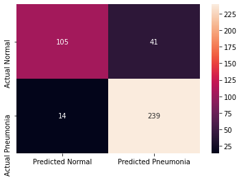
cm = pd.DataFrame(data=confusion_matrix(test_labels[:,0], predictions[:,0], labels=[0,1]),index=["Actual Normal", "Actual Pneumonia"],
columns=["Predicted Normal", "Predicted Pneumonia"])
sns.heatmap(cm,annot=True,fmt="d")
# print the scores for normal and pneumonia categories
print(classification_report(y_true=test_labels[:,0],y_pred=predictions[:,0],target_names =['NORMAL', 'PNEUMONIA']))
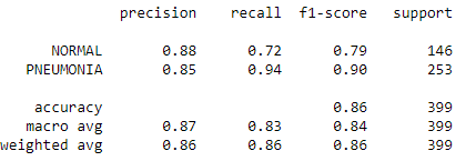
The confusion box shows that the TP and TN predictions are much higher than the FN and FP results. The f1-score for both normal and pneumonia data are 0.79 and 0.9, which are very reasonable too.
Finally, we plot few of the examples of images with percentage of predictions
# print some of the predicted images with percentage of predictions
test_generator.reset()
x=np.concatenate([test_generator.next()[0] for i in range(test_generator.__len__())])
y=np.concatenate([test_generator.next()[1] for i in range(test_generator.__len__())])
print(x.shape)
print(y.shape)
dic = {0:'NORMAL', 1:'PNEUMONIA'}
plt.figure(figsize=(20,14))

#for i in range(0+200, 9+200):
for idx, i in enumerate(np.random.randint(1, 388, 6)):
    plt.subplot(2, 3, idx+1)
    if preds[i, 0] >= 0.5:
        out = ('{:.2%} probability of being Pneumonia case'.format(preds[i][0]))


    else:
        out = ('{:.2%} probability of being Normal case'.format(1-preds[i][0]))
    plt.title(out +"\n Actual case :" + dic[y[i][0]])
    plt.imshow(np.squeeze(x[i]))
    plt.axis('off')
plt.show()
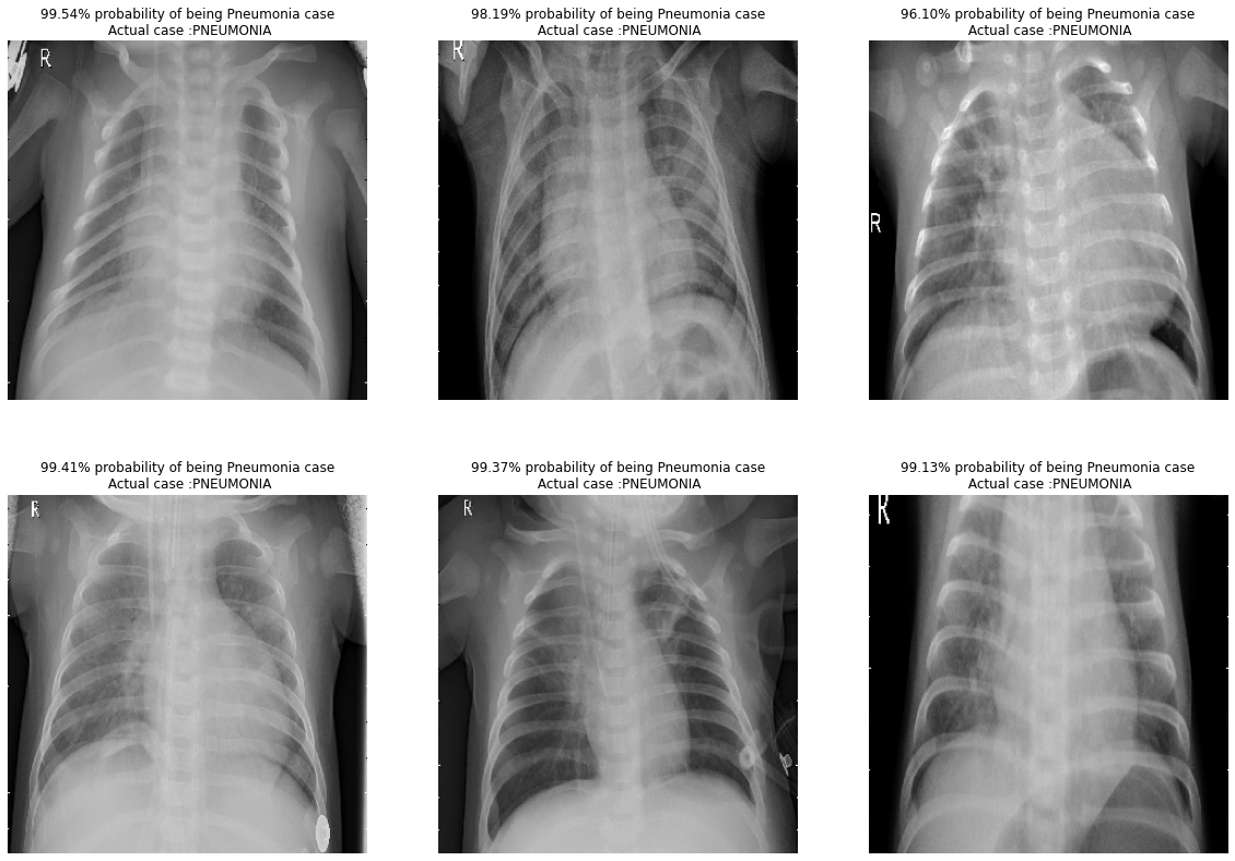
We randomly plot some of the pictures from the test folder and give the prediction and actual case of the picture. The prediction and actual results are identical to each other in our samples.
Conclusion
Based on 20% of the whole dataset, we created a CNN model based on a Pretrained model (VGG19), which can classify X-ray images as Pneumonia cases or Normal cases. The model was then retrained with the whole dataset and tested with the separated test images. The accuracy of the prediction is around 95%.