Phase 3 Project

Project Overview

For this project, I used several regression models to model the data from SyriaTel and predict if their customer will churn the plan or not.

Business Problem

Build a classifier to predict whether a customer will (“soon”) stop doing business with SyriaTel, a telecommunications company. Note that this is a binary classification problem.

Most naturally, your audience here would be the telecom business itself, interested in losing money on customers who don’t stick around very long. Are there any predictable patterns here?

Plan

Since the SyriaTel Customer Churn is a binary classification problem problem, I will try to use several different algorithms to fit the data and select one of the best one. The algorithms I will try include Logistic Regression, k-Nearest Neighbors, Decision Trees, Random Forest, Support Vector Machine. The target of the data we need to fit is the column ‘churn’. The features of the data is the other columns in dataframe. However, when I load the data file into dataframe, i found some of the columns are linear correlated with each other. I need to drop one of them. We need to polish the data first.

Looking at the dataframe, I need to steply polish some features and remove some of the columns:

1. The pairs of features inclued (total night minutes and total night charges), (total day minutes and total night charges), (total night minutes and total night charges), (total intl charge and total intl minutes) are high correlated with each other. I need to remove one in each columns.
2. All the phone numbers are unique and act as id. So it should not related to the target. I will remove this feature.
3. The object columns will be catalized.

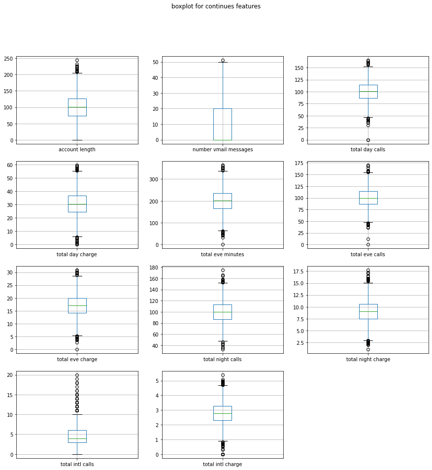
The above figures show that there are multipal columns contain some outlier data. I then collected all the columns and remove the outlier by 1.5 x IQR

to_modify = ['price', 'bedrooms', 'bathrooms', 'sqft_living', 'sqft_lot','sqft_above','sqft_basement']
for col in to_modify:
    Q1 = df_precessed[col].quantile(0.25)
    Q3 = df_precessed[col].quantile(0.75)
    IQR = Q3 - Q1
    df_precessed = df_precessed[(df_precessed[col] >= Q1 - 1.5*IQR) & (df_precessed[col] <= Q3 + 1.5*IQR)]

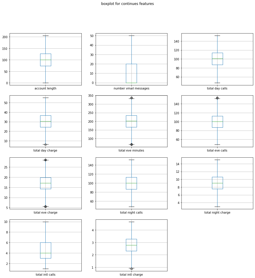
The data looks much better now with very few of outlier numbers.

Now the data was ready and we need to prepare and modeling the data with varies models.

Plan

1. Perform a Train-Test Split

For a complete end-to-end ML process, we need to create a holdout set that we will use at the very end to evaluate our final model’s performance.

2. Build and Evaluate several Model including Logistic Regression, k-Nearest Neighbors, Decision Trees, Randdom forest, Support Vector Machine.

For each of the model, we need several steps

1. Build and Evaluate a base model
2. Build and Evaluate Additional Logistic Regression Models
3. Choose and Evaluate a Final Model

3. Compare all the models and find the best model

1. Prepare the Data for Modeling

The target is Cover_Type. In the cell below, split df into X and y, then perform a train-test split with random_state=42 and stratify=y to create variables with the standard X_train, X_test, y_train, y_test names.

y = df_polished_4['churn'] * 1   #extract target and convert from boolen to int type
X = df_polished_4.drop('churn', axis= 1)
X_train, X_test, y_train, y_test = train_test_split(X, y, random_state=42)

Since the X features are in different scales, we need to make them to same scale. Now instantiate a StandardScaler, fit it on X_train, and create new variables X_train_scaled and X_test_scaled containing values transformed with the scaler.

scale = StandardScaler()
scale.fit(X_train)
X_train_scaled = scale.transform(X_train)
X_test_scaled = scale.transform(X_test)

As the data is inbalanced, I used smote to make the training data balanced before fitting.

smote = SMOTE()
X_train, y_train = smote.fit_resample(X_train_scaled, y_train) 

2. Build and Evaluate several Model

Build the model with Logistic Regression

Log = LogisticRegression(random_state=42)
a = Log.fit(X_train, y_train)

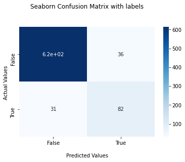
I then plot the confusion matrix for this model

def plot_confusion(model, X_test_scaled, y_test):   
    y_hat_test = model.predict(X_test_scaled)
    
    print('accuracy_score is ', round(accuracy_score( y_test, y_hat_test), 5))
    print('f1_score is ', round(f1_score( y_test, y_hat_test), 5))
    print('recall_score', round(recall_score( y_test, y_hat_test), 5))
    print('precision_score', round(precision_score( y_test, y_hat_test), 5))


    cf_matrix  = confusion_matrix(y_test,y_hat_test)

    # make the plot of cufusion matrix 
    ax = sns.heatmap(cf_matrix, annot=True, cmap='Blues')

    ax.set_title('Seaborn Confusion Matrix with labels\n\n');
    ax.set_xlabel('\nPredicted Values')
    ax.set_ylabel('Actual Values ');

    ## Ticket labels - List must be in alphabetical order
    ax.xaxis.set_ticklabels(['False','True'])
    ax.yaxis.set_ticklabels(['False','True'])

    ## Display the visualization of the Confusion Matrix.
    plt.show()
    
plot_confusion(Log, X_test_scaled, y_test)  

accuracy_score is 0.76832
f1_score is 0.5124
recall_score 0.82301
precision_score 0.372

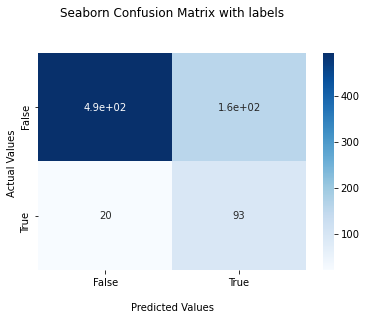
The confusion box shows massive TN data compared to the TP, FP, and FN. In this project, the main focus of our fitting is on TP, which is the customers who will churn the plan. In this case, the accuracy, including the TN data, is not work in our project. However, the f1 score, which combines both recall and precision data, looks well working for our fitting. The confusion box for Logistic Regression fitting shows there is too much FP, and the F1 score is not high enough. Thus the Logistic Regression is not working well for these data.

Build the model with k-Nearest Neighbors

knn_base = KNeighborsClassifier()
knn_base.fit(X_train, y_train)
plot_confusion(knn_base, X_test_scaled, y_test)  

accuracy_score is 0.79058 f1_score is 0.49367 recall_score 0.69027 precision_score 0.38424

The scores for KNeighborsClassifier are pretty high. But the score for traing is higher than testing data. We will try to use other parameter to find the best number of neighbor used for fitting.

#set the list of n_neighbors we will try
knn_param_grid = {
    'n_neighbors' : [1,3,5,6,7,8,9, 10]
}
knn_param_grid =  GridSearchCV(knn_base, knn_param_grid, cv=3, return_train_score=True)
#fit the model to data
knn_param_grid.fit(X_train, y_train)
# find the best parameter
knn_param_grid.best_estimator_

KNeighborsClassifier(n_neighbors=1)

knn_base_best = KNeighborsClassifier(n_neighbors=1)
knn_base_best.fit(X_train, y_train)

plot_confusion(knn_base_best, X_test_scaled, y_test) 

accuracy_score is 0.82068 f1_score is 0.45418 recall_score 0.50442 precision_score 0.41304

For data fit to model with k-Nearest Neighbors, the f1 score is still low because there is a lot of FP data.

Build the model with Decision Trees

DT_baseline = DecisionTreeClassifier(random_state=42)
DT_baseline.fit(X_train, y_train)

plot_confusion(DT_baseline, X_test_scaled, y_test)  

accuracy_score is 0.87696 f1_score is 0.624 recall_score 0.69027 precision_score 0.56934

The f1 score for DT is not high also.

#set the list of parameters we will try

dt_param_grid = {
    'criterion': ['gini', 'entropy'],
    'max_depth': [2, 3, 4, 5 , 10],
    'min_samples_split': [2, 5, 10],
    'min_samples_leaf' : [1, 2, 3, 4, 5, 6]
}
dt_grid_search =  GridSearchCV(DT_baseline, dt_param_grid, cv=3, return_train_score=True)

# Fit to the data
dt_grid_search.fit(X_train, y_train)
# find best parameters
dt_grid_search.best_params_

{‘criterion’: ‘entropy’, ‘max_depth’: 10, ‘min_samples_leaf’: 1, ‘min_samples_split’: 2}

DT_baseline_best = DecisionTreeClassifier(random_state=42, criterion='entropy', max_depth=10,
                                          min_samples_leaf=1, min_samples_split=2)
DT_baseline_best.fit(X_train, y_train)
plot_confusion(DT_baseline_best, X_test_scaled, y_test)  

accuracy_score is 0.9123 f1_score is 0.70996 recall_score 0.72566 precision_score 0.69492

Plot confusion matrix

Compare to the first to model, Decision Tree gives us better f1 score. However, it is still not high enough since FP and FN are still high compare to TP.

Build the model with Support Vector Machine

svm_baseline = SVC()
svm_baseline.fit(X_train, y_train)


plot_confusion(svm_baseline, X_test_scaled, y_test)  

accuracy_score is 0.87696 f1_score is 0.63281 recall_score 0.71681 precision_score 0.56643

#set the list of parameters we will try

svm_param_grid = {
    'C' :[0.1, 1, 5, 10, 100],
    'kernel': ['poly', 'rbf'],
    'gamma': [0.1, 1, 10, 'auto'],
    

}
svm_grid_search =  GridSearchCV(svm_baseline, svm_param_grid, cv=3, return_train_score=True)

svm_grid_search.fit( X_train_scaled, y_train)

svm_grid_search.best_params_

{‘C’: 10, ‘gamma’: 0.1, ‘kernel’: ‘rbf’}

# refit the model to data with best parameters

svm_baseline_best = SVC(C= 10, gamma= 0.1, kernel= 'rbf')
svm_baseline_best.fit(X_train, y_train)

plot_confusion(svm_baseline_best, X_test_scaled, y_test)  

accuracy_score is 0.86911 f1_score is 0.53271 recall_score 0.50442 precision_score 0.5643

Compare to the SVC baseline model, the training score decreased, the testing score is not changing. They are pretty high but still less than DT model. The False negtive rate for this model is also very high.

Build the model with RandomForestClassifier

rf_clf = RandomForestClassifier()
rf_clf.fit(X_train, y_train)

plot_confusion(rf_clf, X_test_scaled, y_test)  

accuracy_score is 0.94241 f1_score is 0.80531 recall_score 0.80531 precision_score 0.80531

rf_param_grid = {
    'n_estimators' : [10, 30, 100],
    'criterion' : ['gini', 'entropy'],
    'max_depth' : [None, 2, 6, 10],
    'min_samples_split' : [5, 10],
    'min_samples_leaf' : [3, 6],
    
}
rf_grid_search = GridSearchCV(rf_clf, rf_param_grid, cv =3)

rf_grid_search.fit(X_train, y_train)
print("")
print(f"Optimal Parameters: {rf_grid_search.best_params_}")

Optimal Parameters: {‘criterion’: ‘entropy’, ‘max_depth’: None, ‘min_samples_leaf’: 3, ‘min_samples_split’: 5, ‘n_estimators’: 100}

rf_clf_best = RandomForestClassifier(criterion='entropy', max_depth=None, min_samples_leaf=3, min_samples_split=5, n_estimators = 100)
rf_clf_best.fit(X_train, y_train)

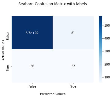
plot_confusion(rf_clf_best, X_test_scaled, y_test)  

accuracy_score is 0.94895 f1_score is 0.83117 recall_score 0.84956 precision_score 0.81356

Compare to other four models, the model of Random Forest gives us best results on the f1 scores. The TP in confusion matrix incresed and the FP, FN decresed. Thus we selected random Forest for our final model.

#### Compare all the models and find the best model, then evaluate it.

The final score for training and testing data are very high and close to each other which suggest there is no overfit or downfit to the trainning data. Now let find out the weight of each features to the target results.

I make Random Forest model to the final one.

importance_DT = rf_clf_best.feature_importances_
col = []
val = []
combine = []
# summarize feature importance
for i,v in zip(X.columns, importance_DT):
    
    combine.append((i, v))
# plot feature importance
plt.figure(figsize = (15, 5))

sort_features =sorted(combine, key = lambda x:x[1])

col = [feat[0] for feat in sort_features]
val = [feat[1] for feat in sort_features]



plt.barh(col, val,  align='center')
plt.xlabel('Feature importance')
plt.ylabel('The features')


plt.show()
for i in range (16 , 11, -1):
    
    print(col[i], val[i])

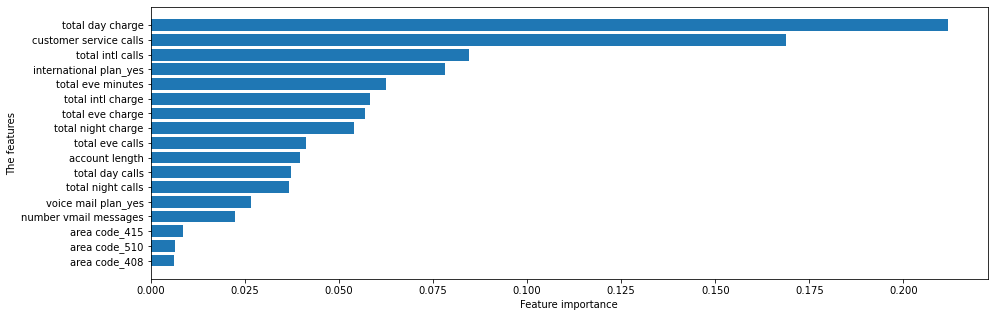
The top 5 important features:

total day charge 0.21184

customer service calls 0.16868

total intl calls 0.0846349709

international plan_yes 0.07813

total eve minutes 0.062427

### Check if there is special patten for the top five important features

# Plot the histogram for total day charge of customers who churned and not churned.

plt.figure(figsize=(15,6))
plt.subplot(1,2,1)
plt.hist(df_polished_4[df_polished_4['churn'] == 1]['total day charge'], density=True)
plt.xlabel('Total day charge')
plt.ylabel('Amount')
plt.title('Churned')


plt.subplot(1,2,2)
plt.hist(df_polished_4[df_polished_4['churn'] == 0]['total day charge'], density=True)
plt.xlabel('Total day charge')
plt.ylabel('Amount')
plt.title('Not churned')
plt.show()

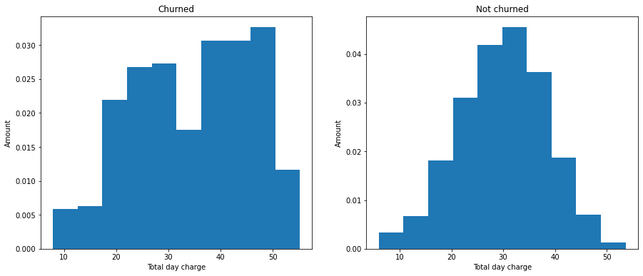
The histograms for customers who churned and not churned show that the total day chare have a lot of overlap with each other.The customers who had total day charg more than 40 have more chance to churn the plan.

Plot the histogram for ‘customer service calls’ of customers who churned and not churned with similar code.

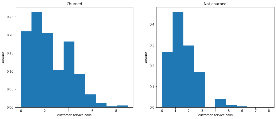
The histogram are similar to each other. However, the customer who had 4 international calls had higher chance to churn the plan.

 
churn = df_polished_4[df_polished_4['churn'] == 1]['international plan_yes'].value_counts(normalize=True)
not_churn = df_polished_4[df_polished_4['churn'] == 0]['international plan_yes'].value_counts(normalize=True)
df_churn = pd.DataFrame([ churn, not_churn ], index =[' No', 'Yes'])
df_churn.columns = ['not churn', 'churn']
print(df_churn)
df_churn.plot(kind = 'bar', xlabel = 'international plan', ylabel = 'Normalized amount')
plt.show()

        not churn     churn

No 0.721198 0.278802

Yes 0.933944 0.066056

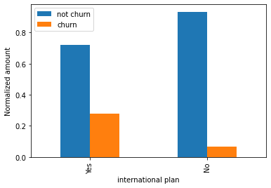
This data show that the customers who have international plan have 27% chance to churn the service. But the customers who do not have the international plan have only 6.7% chance to churn the service.

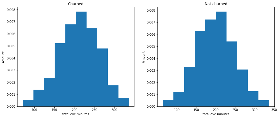
Plot the histogram for ‘total eve minutes’ of customers who churned and not churned.

There is no clear relationship between total eve minutes and churn or not.

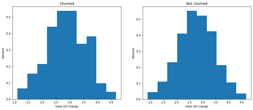
Plot the histogram for ‘total intl charge’ of customers who churned and not churned.

There is no clear relationship between total intl charge and churn or not.

# Conclusion

We polished our original data by removing the outlier and catalyzing the necessary columns. We then tested several models to fit out data and selected the best one, Random Forest. The final score of predicting is 0.83117, which is very high. By plotting the feature importance, we found that the top 5 weighted features are total day charge, customer service calls, international plan_yes, total intl calls, and eve minutes. We then plot the histogram of each feature separated by the customers who churn and not churn the plan. We found that customers who had day charge more than 40 or had customer service call four and more or had an international plan had a higher chance of churning the service. When investigating the features of total day charge and customer service calls, customers using Syriatel service more often have a higher chance of churning the service. Thus, Syriatel company can promote the service charge to attract people to use more of that. They also need to make the customer service friendlier and more professional to help customers address the problems. The international plan is also crucial for customers to churn the service. Based on this point, Syriatel can also make some memorable plans if more customers use the international program.

• ← Previous Post
• Next Post →