Project Overview
For this project, I used regression modeling to analyze house sales in a northwestern county.
The Data
This project uses the King County House Sales dataset, which can be found in kc_house_data.csv in the data folder in this repo. The description of the column names can be found in column_names.md in the same folder. As with most real world data sets, the column names are not perfectly described, so you’ll have to do some research or use your best judgment if you have questions about what the data means.
Business Problem
We have had the house selling records for the last few years. With these data, I want to build a model in which I can use the features in the data about the house to predict the price. In this case, we can guide both the seller and buyer to their business. The seller can use the model to predict the selling price of their house and if they need to do any renovation before selling their home. The buyer can have some suggestions about which kind of house they can afford based on their budget. To the details goal:
- polish the data which have no meaning or is null to the price.
- remove the features which do not contribute to the house price.
- check if there are some high correlated features in which some of them can be removed.
- build the linear regression model.
- check how the features can contribute to the house change.
After reviewing the data, I load the house data in to the dataframe and did some necessary modification
I steply removed and polished most of the columns which is not contribute to the price of house
- The id is not related to the price
- Split the date file to month and year.
- Since the lat and long data is high related to the zipcode, I need to remove them.
- Remodle the zip column with only the first three number
- Remove the sqft_living15 and sqft_lot15 from columns.
- Change the yr_built to the age of house at sold time
- Change the yr_renovated to if the house is renovated and is the renovated within 10 and 30 years at sold.
After the initial data polish, I checked the number of unique value for each of the columns. Some of the columns like price, sqft_living, sqft_lot had more than hundres of unique values which can be consider to be continues values. However, some of the features contain only few unique values.
I then drawed the distribution of each of the columns which had more than 10 unique value to check if there is any outlier values.
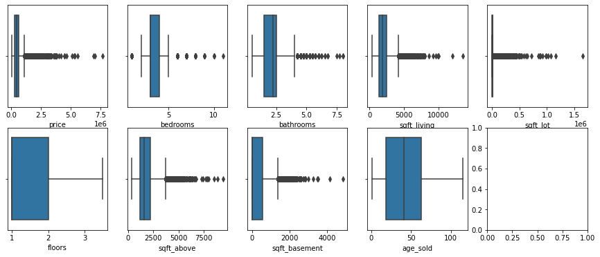
The above figures show that there are multipal columns contain some outlier data. I then collected all the columns and remove the outlier by 1.5 x IQR
to_modify = ['price', 'bedrooms', 'bathrooms', 'sqft_living', 'sqft_lot','sqft_above','sqft_basement']
for col in to_modify:
    Q1 = df_precessed[col].quantile(0.25)
    Q3 = df_precessed[col].quantile(0.75)
    IQR = Q3 - Q1
    df_precessed = df_precessed[(df_precessed[col] >= Q1 - 1.5*IQR) & (df_precessed[col] <= Q3 + 1.5*IQR)]

The data looks much better now with very few of outlier numbers.
In order to check the relationship between the price with most of the columns with few unique numbers, I plot their relations in seperate figures.

The figures show that the house price have clear relationship with all of the features. However, there is few figures are pretty close to each other.
To avoid the high correlated features, I filtered the features and find the pair of features with correlation value between 0.7 and 1.
I tested the pairs of feature with correlation more than 0.70.
df = df_precessed.corr().abs().stack().reset_index().sort_values(0, ascending = False)
df['pairs'] = list(zip(df.level_0, df.level_1))
df.set_index(['pairs'], inplace = True)
df.drop(columns = ['level_0', "level_1"], inplace  = True)
df.columns = ['cc']
df.drop_duplicates(inplace = True)
df[(df.cc>.7) & (df.cc<1)]
pairs CC
(sqft_living, sqft_above) 0.814755
(renovated_30, is_renovated) 0.808098
(month, year) 0.786899
There are three pairs of features high related with each other. I need to remove at least one of the features in each pair. Comparing the last list, I decided to delete the columns sqft_above, renovated_30, year, month.
Since there is some columns with only few number of unique values, I need to catalize the features.
to_cat = ['bedrooms','bathrooms', 'floors' ,'view','condition','grade','zipcode','month',]
df_cat = pd.DataFrame()
for col in to_cat:
    df_cat = pd.concat([df_cat, pd.get_dummies(df_precessed[col], prefix = col)], axis = 1)
to_cat_2 = ['waterfront','is_renovated','renovated_10']
df_cat_2 = pd.DataFrame()
for col in to_cat_2:
    df_cat_2 = pd.concat([df_cat_2, pd.get_dummies(df_precessed[col], prefix = col, drop_first=True)], axis = 1)
df_precessed = df_precessed.drop(to_cat,axis  = 1 )
df_precessed = df_precessed.drop(to_cat_2,axis  = 1 )
df_precessed = pd.concat([df_precessed, df_cat, df_cat_2], axis = 1)
df_precessed.head()
Regression
Until now, I finished the polish of the all the features and then I will split the data to trainning and testing parts to do the fitting.
split the data to training and testing part
from sklearn.model_selection import train_test_split
y = df_precessed['price']
X = df_precessed.drop('price', axis  = 1)
X_train, X_test, y_train, y_test = train_test_split(X, y, random_state=42)
print(len(X_train), len(X_test), len(y_train), len(y_test))
Next, I start to build the regression model
Build a Model with All Numeric Features
from sklearn.linear_model import LinearRegression
from sklearn.model_selection import cross_validate, ShuffleSplit

baseline_model = LinearRegression()


splitter = ShuffleSplit(n_splits=3, test_size=0.25, random_state=0)
model = LinearRegression()

model_scores = cross_validate(
    estimator=model,
    X=X_train,
    y=y_train,
    return_train_score=True,
    cv=splitter
)

print("Current Model")
print("Train score:     ", model_scores["train_score"].mean())
print("Validation score:", model_scores["test_score"].mean())
print()
)
Current Model Train score: 0.5897185649583689 Validation score: 0.5858295197121807
The score for the trainning and testing data are very similar to each other and not bad. Hoever, some of the features might not be suitable for the linear regression. I then tried to selecting Features with sklearn.feature_selection.
Select the Best Combination of Features
I checked the linear regression fitness for all the features first.
from sklearn.feature_selection import RFECV
from sklearn.preprocessing import StandardScaler

# Importances are based on coefficient magnitude, so
# we need to scale the data to normalize the coefficients
X_train_for_RFECV = StandardScaler().fit_transform(X_train)

model_for_RFECV = LinearRegression()

# Instantiate and fit the selector
selector = RFECV(model_for_RFECV, cv=splitter)
selector.fit(X_train_for_RFECV, y_train)

# Print the results
print("Was the column selected?")
for index, col in enumerate(X_train.columns):
    print(f"{col}: {selector.support_[index]}")
The results show that all of the features are necessary for the regression.
I then did the linear regression with OLS.
import statsmodels.api as sm

sm.OLS(y_train, sm.add_constant(X_train)).fit().summary()


Results The Coefficient of all the features show how each of the feature affect the house price. Briefly, for the house size, the sqft_living had value 114.5637 which suggests that increasing 1 sqrt of living area, the house pirce will increase 114 dollars. However, the sqft_lot and sqft_basement had negtive correlation to the house price even though the correlation value is very low compare to sqft_living. The number is bedrooms had negtive negtive correlation to the house price. More bathrooms, floors, views and conditions will increase the house price in general. Grade 4-7 decrease the house price and Grade 8-10 increase the house price a lot by around 500000 each level. To the zipcode, the house in some area is much higer than others. The house price in month March to July is obviously higher than other months. If there is what front, the house price will increase by 128000. If the house is renovated, the house price can increasing arount 7540. If the renovated is within 10 years, the house price can increase around 51400.
Validation
I build again the finial model.
X_train_final = X_train[select_cat]
X_test_final = X_test[select_cat]


final_model = LinearRegression()

#Fit the model on X_train_final and y_train
final_model.fit(X_train_final, y_train)

#Score the model on X_test_final and y_test
#use the built-in .score method
final_model.score(X_test_final, y_test)
0.5771902162157758
import the mse to check the mse value
from sklearn.metrics import mean_squared_error

mean_squared_error(y_test, final_model.predict(X_test_final), squared=False)

#check the distribution of price in test data
y_test.hist(bins = 100)
y_test.mean()

The mse value is 123127. The mean of the price is 445683.
This means that for an average house price, this algorithm will be off by about $130331 thousands. Given that the mean value of house price is 445683, the algorithm can patially set the price. However, we still want to have a human double-check and adjust these prices rather than just allowing the algorithm to set them.
For the validation, I first plot the scatter plot of Predicted Price vs the Actual Price
preds = final_model.predict(X_test_final)
fig, ax = plt.subplots(figsize =(5,5))

perfect_line = np.arange(y_test.min(), y_test.max())
#perfect_x = [0, 1]
#perfect_y = [0, 1]

#ax.plot(perfect_x, perfect_y, linestyle="--", color="black", label="Perfect Fit")
ax.plot(perfect_line,perfect_line, linestyle="--", color="black", label="Perfect Fit")
ax.scatter(y_test, preds, alpha=0.5)
ax.set_xlabel("Actual Price")
ax.set_ylabel("Predicted Price")
ax.legend();

I then tested the residuals by qqplot
import scipy.stats as stats
residuals = (y_test - preds)
sm.graphics.qqplot(residuals, dist=stats.norm, line='45', fit=True);

fig, ax = plt.subplots()
ax.scatter(preds, residuals, alpha=0.5)
ax.plot(preds, [0 for i in range(len(X_test))])
ax.set_xlabel("Predicted Value")
ax.set_ylabel("Actual - Predicted Value");

The validation of prediction and real data shows that the prediction price for most house whose price is low (20% of the max price) is close to the real price. qqplot showes that the house price is well predicted when the house price is not very high. However, for the high value price house, the prediction is not very acturate. There is a lot of shift of prediction price when the house value increase especialy when house price is more than 2 million.
Summary
The Coefficient of all the features show how each of the feature affect the house price. Briefly, for the house size, the sqft_living had value 114.5637 which suggests that increasing 1 sqrt of living area, the house pirce will increase 114 dollars. However, the sqft_lot and sqft_basement had negtive correlation to the house price even though the correlation value is very low compare to sqft_living. The number is bedrooms had negtive negtive correlation to the house price. More bathrooms, floors, views and conditions will increase the house price in general. Grade 4-7 decrease the house price and Grade 8-10 increase the house price a lot by around 500000 each level. To the zipcode, the house in some area is much higer than others. The house price in month March to July is obviously higher than other months. If there is what front, the house price will increase by 128000. If the house is renovated, the house price can increasing arount 7540. If the renovated is within 10 years, the house price can increase around 51400.
To the buyer, We had our prediction model which can predict the house price and give buyer some suggestion about the price they want. However, the predicted house price is higher than the selling price when the price is over 700000. To the seller, our model give them some suggestion how to increase the potential selling value. For example, they can try to renovate the house and make water front if possible and increas the grade of the house.